Quickstart
Construction rules
Boundary conditions (bc) – Rules raising BoundaryConditionError exception if not respected:
bc of the domain must be a combination of ‘ZRAPW’ as for (Z)impedance, (W)all, (A)bsorbing, (R)adiation, and (P)eriodic
bc of each Obstacle object must be a combination of (Z)impedance, (W)all, (V) velocity
If periodic (P) is chosen as boundary condition for an edge of the domain, ‘P’ must also be chosen as boundary condition for the edge facing it
Grid construction – Rules raising GridError exception if not respected:
The number of points of the PML must be larger than this of the stencil, otherwise GridError exception will be raised
Origin of the domain must be in the domain
For curvilinear meshes, geometric conservation laws must be verified (variable change must remains soft)
Obstacle location – Rules raising CloseObstacleError exception if not respected
Two obstacles cannot be close to a distance of less than twice the size of the stencil that has been declared (11 by default) except if they have a common edge
An obstacle cannot sit astride an (A)borbing subdomain and a regular subdomain
If an obstacle is located inside an (A)bsorbing subdomain (whose width is defined by Npml), an edge of this obstacle must correspond to the edge of the domain.
Creation of set of obstacles
Domain and Obstacle objects can be used to create sets of obstacles.
Use Obstacle to create an obstacle:
First argument is a list of coordinates as [left, bottom, right, top]
Second argument is the boundary conditions [(W)all, (V) velocity, (Z)impedance]
Use Domain to gather all Obstacle objects:
First argument is the shape of the grid (tuple)
Keyword argument data is a list of Obstacle objects
For instance:
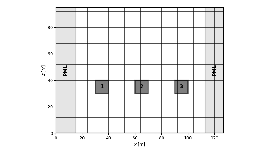
from fdgrid import Mesh, Obstacle, Domain

def custom_obstacles(nx, nz):

    geo = [Obstacle([30, 20, 40, 40], 'WWWW'),
           Obstacle([60, 20, 70, 40], 'WWWW'),
           Obstacle([90, 20, 100, 40], 'WWWW')]

    return Domain((nx, nz), data=geo)

nx, nz = 128, 64
dx, dz = 1., 1.
ix0, iz0 = 0, 0
bc = 'AWAW'

mesh = Mesh((nx, nz), (dx, dz), (ix0, iz0), obstacles=custom_obstacles(nx, nz), bc=bc)
mesh.plot_grid(pml=True)
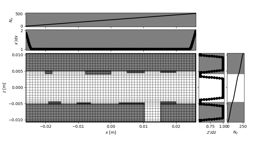
Adaptative mesh example
from fdgrid import AdaptativeMesh, templates


shape = (512, 256)  # Dimensions of the grid
steps = (1, 1)              # grid steps
ix0, iz0 = 0, 0             # grid origin
bc = 'WWWW'                 # Boundary conditions : left, bottom, right, top.
                            # Can be (W)all, (A)bsorbing, (P)eriodic, (Z)impedance, (R)adiation

# Set up obstacles in the grid with a template
obstacles = templates.street(*shape)

# Generate AdaptativeMesh object
msh = AdaptativeMesh(shape, steps, (ix0, iz0), obstacles=obstacles, bc=bc)

# Show
msh.plot_grid(axis=True, N=8)
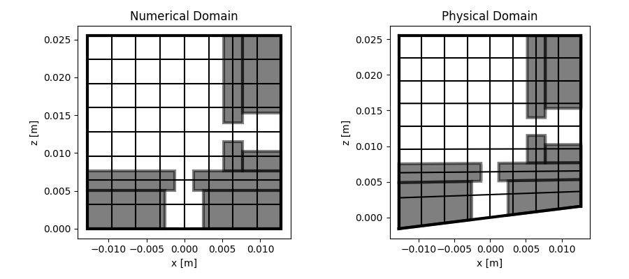
Curvilinear mesh example
from fdgrid import CurvilinearMesh, templates
import numpy as np

shape = (256, 256)       # Dimensions of the grid
steps = (1e-4, 1e-4)     # grid steps
origin = (128, 0)        # grid origin
bc = 'WWWW'              # Boundary conditions : left, bottom, right, top.
                        # Can be (W)all, (A)bsorbing, (P)eriodic, (Z)impedance, (R)adiation

# Set up obstacles in the grid with a template
obstacles = templates.helmholtz_double(*shape)

# Setup curvilinear transformation
def curv(xn, zn):
    dx = xn[1] - xn[0]
    f = 5*dx
    xp = xn.copy()
    zp = zn + np.exp(-np.linspace(0, 10, zn.shape[1]))*np.sin(2*np.pi*f*xn/xn.max()/2)
    return xp, zp

# Generate CurvilinearMesh object
msh = CurvilinearMesh(shape, steps, origin, obstacles=obstacles, bc=bc, fcurvxz=curv)

# Show physical grid
msh.plot_physical()
Mesh with moving boundaries
Obstacle instances inherit the set_moving_bc method. This method allows you to set moving edges. set_moving_bc can take as many arguments as the number of V boundaries. Each of these arguments must be a dictionary with the following keys :
f: the oscillation frequency
A: the oscillation amplitude
phi: the phase of oscillation
profile: the oscillation profile of the boundary. For now, it can be ‘sine’ (sine profile), ‘tukey’ (tapered cosine profile)
func : function describing the time evolution of the bc
kwargs: special arguments than can be passed to profile:
for ‘tukey’, can be ‘alpha’, the shape parameter (between 0 and 1)
for ‘sine’, can be ‘n’, the period fraction (1 stands for a complete period, 2 for half a period)
An example is given below:
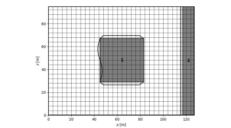
from fdgrid import Mesh, Obstacle, Domain

def custom_obstacles(nx, nz, size_percent=20):

    size = int(min(nx, nz)*size_percent/100)

    obs1 = Obstacle([int(nx/2)-size, int(nz/2)-size, int(nx/2)+size, int(nz/2)+size], 'VVWV')
    obs2 = Obstacle([nx-11, 0, nx-1, nz-1], 'VWWW')

    obs1.set_moving_bc({'f': 70000, 'A': 1, 'profile': 'sine', 'kwargs': {'n': 1}},
                       {'f': 30000, 'A': -1, 'profile': 'tukey', 'kwargs': {'alpha':0.2}},
                       {'f': 30000, 'A': 1, 'profile': 'tukey', 'kwargs': {'alpha':0.2}})
    obs2.set_moving_bc({'f': 73000, 'A': -1, 'profile': 'tukey'})

    return Domain((nx, nz), data=[obs1, obs2])


nx, nz = 128, 96
dx, dz = 1., 1.
ix0, iz0 = 0, 0
bc = 'WWWW'

mesh = Mesh((nx, nz), (dx, dz), (ix0, iz0), obstacles=custom_obstacles(nx, nz), bc=bc)
mesh.plot_grid(pml=True, legend=True, bc_profiles=True)