Microscopy : Fundamentals

The main problem with image formation under very high numerical apertures is the very high inclination of the involved optical rays. Numerical apertures of \(0.70\) ; \(0.95\) (in air) or \(1,30\) (in immersion oil) lead to extreme rays making with the optical axis angles of (respectively) \(45°\), \(72°\) and \(59°\) ! Therefore, we are far from the Gauss conditions and the domain where approximate stigmatism can be used. To obtain high quality images, one needs to work with optical conjugations that are rigorously stigmatic and aplanetic. Thus, when designing microscopes objectives, curvature centers and Weierstrass points of the involved spherical surfaces are of great use.

Remark : These objectives are based on the aplanetic meniscus of Amici (see fig. below). The object is located at the curvature center of the first surface. Its image (superimposed to the object) is located at the real Weierstrass point of the second surface, which creates an expanded virtual image of the object seen under a smaller numerical aperture.

Therefore, for each particular microscope objective, the pair of points object/image is fixed. Moreover, simple planar interfaces may have a significant influence on the imaging quality, as shown in the following paragraph.

Most microscopic samples observed in transmission are protected by a thin glass slide with planar and parallel surfaces called coverslip^[1]. This coverslip has an optical power equal to zero but still affects the oblique rays that are going through it (lateral displacement). This phenomenon increases when the inclination of the rays increases, which translates into a loss of stigmatism, as shown on figure 4 (introduction of spherical aberrations).

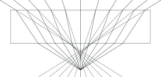
We usually consider that the coverslip significantly affects the observed image quality as soon as the objective numerical aperture exceeds \(0.30\). For numerical apertures larger than \(0.70\), image deterioration is obvious and sometimes a serious problem.

However, it is possible to solve this problem by introducing within the objective (by a judicious design) an aberration that will exactly compensate to the one introduced by the coverslip. One must realize, however, that such an objective will give a bad image of a sample with no coverslip. Manufacturers generally offer two versions of all their objectives of numerical aperture larger than \(0.30\), one to work with a coverslip and one to work without a coverslip. This latter version is usually dedicated to the so called metallographic microscopes, where opaque objects are observed using back illumination through the objective (see Fig.12, in the supplements, at the end of this course). The particular version intended is identified by an inscription on the objective mount (see the subsection « objectives labeling »).

It is possible to qualitatively observe this phenomenon by using as the object a slide covered with a thin aluminum layer, with small holes in this layer. These holes, illuminated using Köhler illumination, will serve as point-like light sources on a dark background, and will allow observing the objective point-spread function. For a perfect objectif and perfect focusing, the point-spread function is an Airy pattern. Otherwise, the observed pattern and most of all its evolution with focusing give information about the system quality. This (classical) method for measuring the aberrations of an optical system is called “bright point method”. The point-spread functions of a perfect system (column a) and of a system with spherical aberration (column b) are shown on figure 5 for several focus up and below the paraxial image.

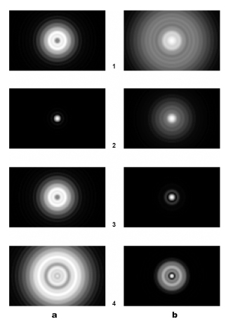
From one row to the next, the focusing is varied of the same distance. The paraxial image corresponds, for both columns, to the second row. The image a2 therefore represents the Airy pattern. In presence of spherical aberrations, the best focusing does not correspond to the paraxial image. The best point-spread function obtained in this case (image b3) exhibits secondary rings of intensity far superior to the ones of the Airy pattern, which explains the image blurring obtained with such an aberrating system. Please note the point-spread function symmetry with respect to the plane of best focusing obtained in the case of an aberration-free system (column a). With spherical aberration (column b) this symmetry is completely lost, and the point-spread functions obtained before and after the plane of best focusing (b3) greatly differ in shapes.

Using rigorously stigmatic optical conjugations, such as the Weierstrass points, when designing the microscope objectives, requires that the intermediate image observed with the eyepiece to be at a precise location, fixed with respect to the objective. Focusing should therefore be obtains by varying the distance object/objective, keeping the distance objective/eyepiece fixed. A microscope should thus work like an optical viewfinder with a fixed working distance. To allow for a certain interchangeability of the microscope components (objectives, eyepieces...) between various manufacturers, several precise dimensional standards have been defined for the microscope ( ISO TC172 [8036 à 8040 + 8255 + 8578...] ). The main ones are shown on Fig. 6 below [ ^[3]].

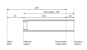
The intermediate image plane must therefore be \(10~ mm\) below the eyepiece support and the object plane \(45~mm\) below the objective support ¹ . The tube length (i.e. the distance between the eyepiece and objective supports) has a normalized value of \(160~mm\). However, it is possible to find other tube lengths: for example, older metallographic microscopes have a tube length of \(230~mm\). But more importantly, a certain type of objective corrected for an infinite tube length (or, in short, corrected for ∞), is offered by most manufacturers for high quality equipment. These objectives are designed to image the object at infinity without aberration. This distance is brought back to a finite distance by an additional converging optical system, called tube lens ² , located in the microscope stand. A real image is therefore formed, equivalent to the intermediate image of “conventional microscopes”, and observed with the eyepiece. With this set-up, it is easier to design and insert additional components in the optical path, which is useful for the techniques using contrast or for reflected light illumination.

The key point is that a slide with parallel surfaces, even curved, does not introduce aberration for (and only for) objects located at infinity (see the two supplement pages at the end of that course grain).

Considering the multiplicity of existing configurations, the user must be very careful in using the right objectives with the right microscope³. To help him in this task, the length of the matching tube lens is usually engraved in the objective mount.

As was just mentioned, there are plenty of available objectives, even within a single manufacturer. To help the user, several useful characteristics are always engraved on the objective mounts, naming: the objective magnification⁴, numerical aperture, immersion medium (if different from air), the coverslip thickness and the length of the tube lens (in mm) for which the objective is corrected. This information is usually complemented with a reference, specific for each manufacturer, which identifies the objective “class” (see the next subsection about “microscope objective classes”).

This information is usually mentioned in the following way, together with eventual additional indications specific to each manufacturer and objective series:

Here are some examples extracted from objective catalogs of several manufacturers:

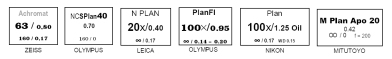
Immersion medium are usually listed as follows: \(Oil\) for immersion oil (\(n \simeq 1,517\) à \(588~nm\)), \(W\) for water and \(Gly\) for glycerin. On very old -french- objectives it is possible to find the label \(ih\) (for homogen immersion), also referring to oil immersion objectives.

We also remind the reader that the indication (\(\times Z\)) engraved on the eyepiece mount is its angular magnification factor. Sometimes this number is followed by a second number, called field number, which gives the diameter, in millimeters, of the effectiv observed area of the intermediate image (this number ranges from \(18\) for a low-cost eyepiece to \(26\) for a very high-quality eyepiece, and is usually around \(22\); of course, the objective must also be matched with the eyepiece). On another note, a symbol representing eyeglasses or the letter \(L\) means that the eyepiece has an exit pupil located far enough to be comfortably used with correction eyeglasses.

Ideally, a microscope objective should give a diffraction limited image everywhere within the observed field. Such a property of course. Comes at a cost and is not always necessary for all microscopy applications. This explains why most manufacturers offer three or four “classes” of objectives, achieving various performances and at various prices. Those classes can slightly vary depending on the manufacturer and are usually listed as follows:

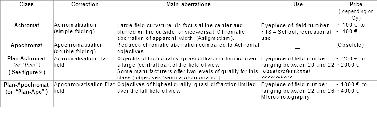
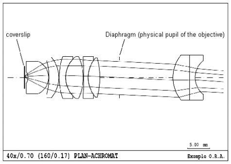
On figure 9, we show an example of optical configuration for an objective \(×40\) of medium quality (type "Plan-Achromat").