Animations
|
|
Animations |
|
 acoustics
animation page
acoustics
animation page

|
The solution of
the wave equation, written in spherical coordinates (r,
 , , ) ) 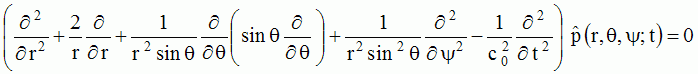 , ,can be written,
for the solutions with separated variables of the form
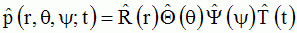 , ,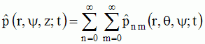 with with
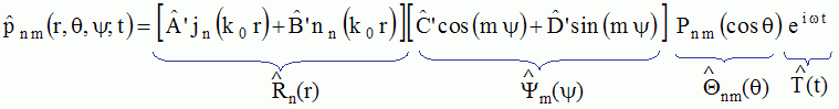 where the
functions jn and nn
are respectively the spherical Bessel functions of the 1st kind and the
spherical Neumann functions, nth-order, and where the functions Pnm(cos
) are the
associated Legendre functions, which can be expressed as a
function of Legendre
polynomials of degree n, denoted Pn,
as following (do not confuse functions Pnm and
polynomials Pn):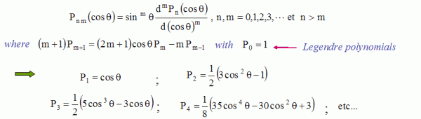 The functions
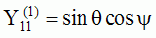
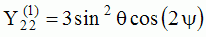
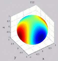
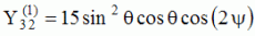
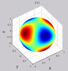
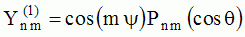 and and 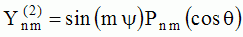 are called "spherical harmonics". are called "spherical harmonics".Hence, for any given n and m, any given solution coming from the separation of variable methods has a structure which is well determined on the unit sphere (parameters and ).
This structure is given by the spherical harmonics, which are orthonormal functions and which form a basis of the
considered space ( ,).These solutions express a complex directivity of the fields which are emitted in an infinite space, by a set of "localised" sources with complex properties. |
|
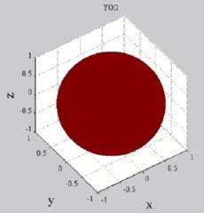
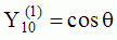
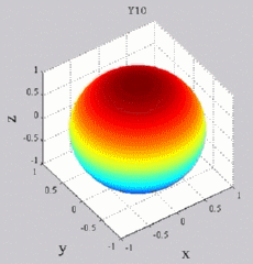
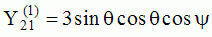
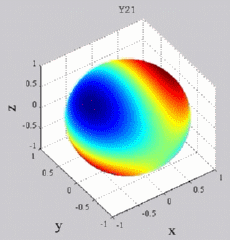
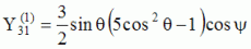
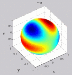
The
animations below present the variations as a fucntion of time, of the
first spherical harmonics  multiplied by the function cos(
 t),
and visualized on the unit sphere, with
color levels (red = maximum, blue = minimum). t),
and visualized on the unit sphere, with
color levels (red = maximum, blue = minimum). |
  |
  |
  |
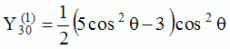  |
| "Zonal"
harmonics: m=0 "Sectoral" harmonics: n=m |
  |
  |
  |
| "Tesseral"
harmonics: 0<m<n |
  |
  |
  |
 Version
française
Version
française