PROPAGATION OF MODAL WAVES IN A ROUGH WAVE GUIDE - MODAL COUPLINGS
 Version
française
Version
française 

|
|
PROPAGATION OF MODAL WAVES IN A ROUGH WAVE GUIDE - MODAL COUPLINGS Version
française |
|
| In collaboration with Laboratoire
d'Acoustique
Ultrasonore
et d'Electronique
(LAUE), UMR CNRS
6068, Le Havre, France
 and the Institut
d'Electronique,
de Microélectronique
et de Nanotechnologie
(IEMN), UMR CNRS 8520 , Lille, France
 in the frame of
the GDR
2501 "Study of the ultrasonic
propagation in non homogeneous media for non destructive testing" ("Etude de la propagation
ultrasonore en milieux non-homogènes en vue du
contrôle non destructif" in french).
|
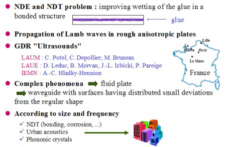 |
A Non Destructive Evaluation and Testing problem
- of plates having an irregular surface condition, - of corrosion, - of quality of bonding in a structure, has led the Research Group (GDR in french) 2501 of CNRS "Study of the ultrasonic propagation in non-homogeneous media for non destructive testing" to study the propagation in anisotropic solid [A16], then fluid, waveguides, with non regular shape profile boundaries (roughness or corrugation). According to the size and to the frequency, this last study [A15, A17] can be applied to other fields, including urban acoustics for instance (propagation in U streets, tunnels, ...). |
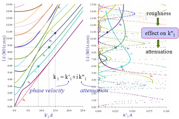
Figure 1 :
Dispersion curves for Lamb modes in a shot blasted glass plate. On the left)
frequency as a function of the real part of the wave number, on the right)
frequency as a function of the imaginary part of the wave number. This
imaginary part is zero when there is no roughness.
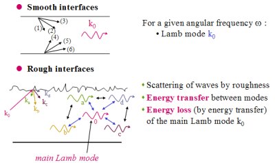 Fig. 2 Fig. 2 |
 and a given wave number k0, there is a reciprocal conversion between the six plane waves and the Lamb mode. and a given wave number k0, there is a reciprocal conversion between the six plane waves and the Lamb mode.When
the interfaces are rough, there is a scattering of all the waves by the
roughness. Let us take one of the six waves, with the wave number k0 corresponding
to the Lamb mode without roughness (figure 2). When impacting on the
roughness, the scattering of this wave creates other Lamb modes by coupling, with different wave numbers (ka, kb, kc, kd, ...). Due to the roughness, while all the waves are propagating, the energy of the main Lamb mode k0 is transfered between all the possible modes (and inversely), which can be expressed in terms of energy loss of the main Lamb mode k0, and therefore by a decreasing
of its amplitude.
|
 Figure 3 : Observation at point  1 of the scattering phenomenon of an acoustic mode on the roughness (total depth of the roughness denoted 1 of the scattering phenomenon of an acoustic mode on the roughness (total depth of the roughness denoted H( )).
The first square bracket represents the field which propagates in the direction of increasing (summation of
the primary wave and of "upstream" coupled waves); the second square
bracket represents the backscattered waves from 1 to + infinity.Click on the image for a zoom |
Qualitatively, when the guide is a fluid waveguide,
and without taking into account the intermodal coupling (only one mode
is considered here), the 1st-order amplitude of the acoustic pressure
(denoted
 ) makes appear the primary wave exp(-ik1m 1) which propagates when the interfaces are smooth, and the coupling due to the scattering of this primary wave on the roughness, which leads to a reallocation of the acoustical energy having the same modal behaviour. ) makes appear the primary wave exp(-ik1m 1) which propagates when the interfaces are smooth, and the coupling due to the scattering of this primary wave on the roughness, which leads to a reallocation of the acoustical energy having the same modal behaviour.
The primary wave and the coupling waves arrive at the observation point
1. The coupling waves are those generated upstream 1 and which propagate in the same direction as the primary wave, and those generated downstream 1 which are backscattered (in
red on figure 3). The waves indicated in green on figure 3 do not contribute to the pressure field at the observation point 1. The details of the calculus can be found in Ref. [A15]. See also figures 9 to 11. |
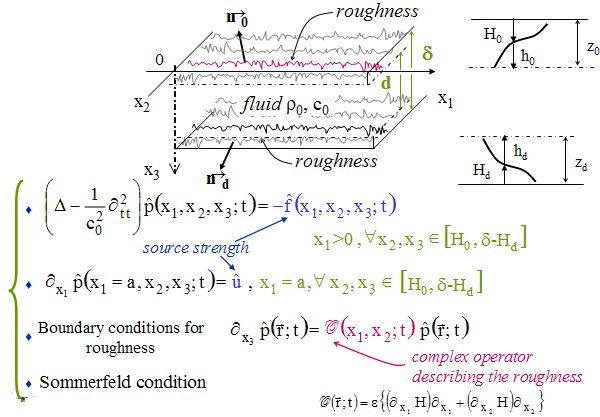 Figure 4 : Geometry of the problem and associated equations Click on the image for a zoom |
The fluid waveguide presented on figure 4 (density
 0 and speed of sound c0,
is bounded by two dimensional shape perturbations (depth H0 from x3=0 and depth Hd from x3= 0 and speed of sound c0,
is bounded by two dimensional shape perturbations (depth H0 from x3=0 and depth Hd from x3= ). The presence of this roughness (total depth H=H0+Hd) leads to define two characteristic thicknesses: that of the "interior guide" d and that of the "outer guide" . The associated eigenvalue problem will be subsequently considered is the Neumann problem associated to this outer guide . ). The presence of this roughness (total depth H=H0+Hd) leads to define two characteristic thicknesses: that of the "interior guide" d and that of the "outer guide" . The associated eigenvalue problem will be subsequently considered is the Neumann problem associated to this outer guide . The well-posed problem is the following.
- propagation equation with bulk source strength, - boundary conditions
expressed by a relationship between the normal derivative of the acoustic
pressure and the acoustic pressure itself, which involves a complex operator
 which describes any type of roughness (derivative operator with respect to x1 and x2,
and function of the derivative of the profile, thus of
the slope), which describes any type of roughness (derivative operator with respect to x1 and x2,
and function of the derivative of the profile, thus of
the slope), - Sommerfeld radiation condition following the directions of propagation. Subsequently, the profile variations (ratio depth H to thickness
and also slopes) are assumed to be small.
|
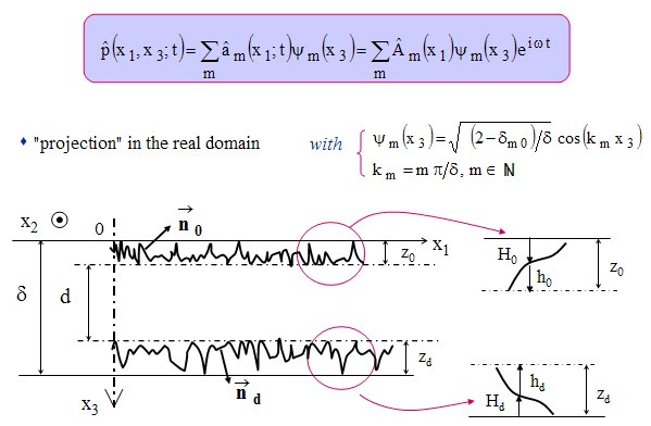 Figure 5 Click on the image for a zoom |
Expansion of the acoustic pressure on the transverse eigenmodes of the guide.
The method is based on the "projection" of the propagation equation on the transverse eigenmodes of the guide. The one dimensional eigenmodes (following x3 coordinate) are those of the 3D dimensional guide bounded by the smooth outer plane surfaces (thickness
). It
should be noted that a "multimodal method" can be
found in the literature. This method utilizes a modal basis which is
different at each point x1;
this modal basis is thus a local basis associated to the real domain.
The present method, called "inter-modal method", utilizes a unique modal basis, using the distance of the outer waveguide which encloses the corrugated considered waveguide (eigenfunctions  m and associated wave numbers km), the "projection" (the integration) being done on the real domain. m and associated wave numbers km), the "projection" (the integration) being done on the real domain. |
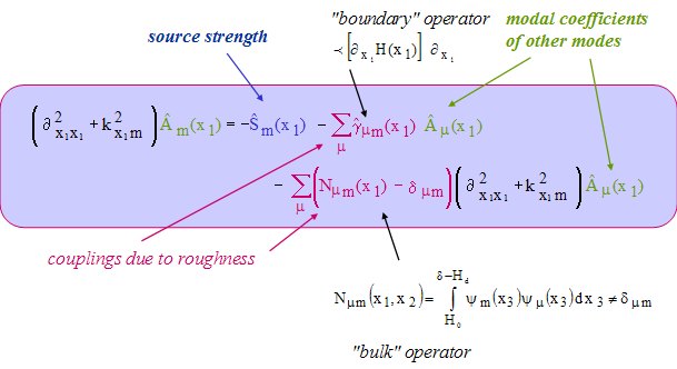 Figure 6 : Use of the Green theorem. Click on the image for a zoom |
Modal formulation Equation
given on figure 6 (particular case of a
monochromatic source) is obtained by the projection of the propagation equation onto
the eigenfunctions
m, then by the use of the 1D Green theorem
which involves the boundary conditions (figure 4). This equation makes appear the modal
coefficients of mode m (in green) and also those of the other modes
µ (created by coupling), the source strength term (in blue), and
two coupling terms (in red): one is related to a boundary operator which includes the slope of the profile and a spatial derivative operator, and the other is related to a "bulk" operator, since the integration takes place over the perturbed lateral dimensions of the guide. |
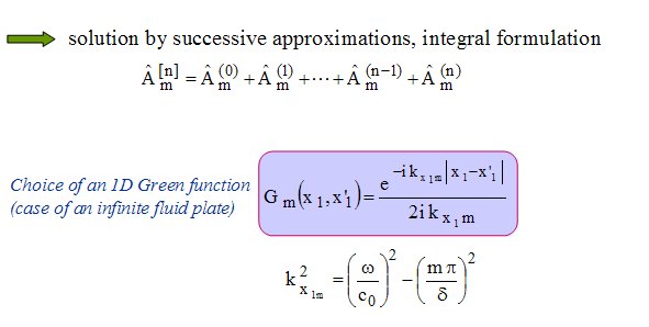 Figure 7 : Solution using integral formulation (1/2).
Click on the image for a zoom |
Solution using integral formulation The solution is obtained by carrying out successive approximations, using at each stage the integral formulation with an appropriate Green function.
In
the case of a semi-infinite plate, and assuming a monochromatic source
flush-mounted at x1=0 and x2=0, the chosen 1D Green function is given
on figure 7.
|
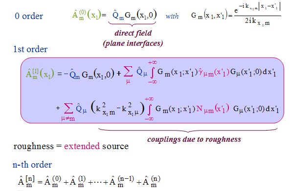 Figure 8 : Solution using integral formulation (2/2).
 Click on the image for a zoom |
Intermodal couplings
- At zero-order, the solution is just the incident field which is the only field which exists when the interfaces are smooth. - At 1st-order, other terms appear, which represent the intermodal coupling effects, due to the roughness,
all over the length of the corrugation. The integrals from -infinite to
+infinite show that the coupling source (here the roughness) acts as a
secondary extended source. Moreover, the expression of the Green
function (figure 7) highlights the fact that the effect of the
corrugation at the
observation point x1 of the coupling upstream and downstream this point is not the same.
It should be noted that the system of equations
(µ,m) is not a linear system because of the presence of the
integrals which represent the non local effect of the roughness; this
is the reason why the solution makes use of the perturbation theory.
- And so on until the nth-order. |
 Figure 9 : Direct mono-mode solution (1/3).
Click on the image for a zoom |
Mono-mode direct solution (out of sources) In
the particular case of a single mode, that created by the source and
numbered m (intermodal couplings µ are neglected), the
equation on figure 6 takes the form of that on figure 9 (the source
strength term cancel because it is assumed to be out of the observation
domain). This particular case is just a qualitative model
is order to provide (in particular) a very simple analytic solution
which helps to understand the physical phenomena : the mode m is
coupled to itself, through the factors indicated in red in the equation
at the bottom of figure 9.
|
 Figure 10 : Direct mono-mode solution (2/3).
Click on the image for a zoom |
Mono-mode direct solution (continuation)
A first-order expansion as a function of the total height of the roughness H=H0+Hd, then a change of the variable x1 --> 1 (translation to the lower order) permit to obtain the framed equation
on figure 10. This equation is truncated only to the 1st order
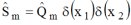
expansion with respect to the small quantity H/. The approximate solution, denoted , can be written as  , , is the zero-order expansion solution (Born approximation). is the zero-order expansion solution (Born approximation).Finaly, the 1st-order perturbation term  is solution of the ordinary differential equation is solution of the ordinary differential equation 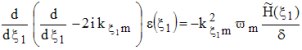 , , |
 Figure 11 : Direct mono-mode solution (3/3). Scattering phenomena of a single mode on the corrugation: a sensor, located at point
1 receives
the primary waves, and the coupled waves which are created upstream and
downstream from this point by scattering on the roughness. Click on the image for a zoom |
Mono-mode direct solution (continuation)
Finaly, the 1st-order acoustic pressure amplitude makes appear the primary wave exp(-ik1m 1) which propagates when the interfaces are smooth, and the coupling due to the scattering of this primary wave on the roughness, which leads to a reallocation of the acoustical energy having the same modal behaviour (since this is here a mono-mode approach).
The primary wave and the coupling waves arrive at the observation point
1. The coupling waves are those generated upstream 1 and which propagate in the same direction as the primary wave, and those generated downstream 1 which are backscattered (in
red on figure 3). The waves indicated in green on figure 3 do not contribute to the pressure field at the observation point 1. This
little qualitative model, which does not take into account the
intermodal coupling, just permits to highlight the basic physical
phenomena. See also figures 2 and 3. |
 Figure
12 : Intermodal couplings in the particular case of a sawtooth periodic
profile. The modes created by coupling due to the roughness are denoted µ and the mode generated by the source is denoted m.
Click on the image for a zoom |
Intermodal couplings - Particular case of a periodic sawtooth profile (spatial period
 ). ).Four modes are taken into account here, the mode µ=3 being evanescent for the chosen frequency. The order n=3 is generally enough in order to make the model converge. The results are presented on figures 13 to 17. The phonon relationships (see figure 18 and associated text) permit to predict either a strong or a weak coupling between the modes, and also the oscillation periods. |
 Figure 13 : Modulus
of the acoustic pressure amplitude of the mode µ=0 created by
coupling. The period of the periodic oscillations involves the spatial
period
of the profile, and the wave numbers of each mode (see phonon relationship).Click on the image for a zoom |
 Figure 14 : Modulus of the acoustic pressure amplitude of the mode m=1 created by the source. The coupling due to the roughness creates other modes than the mode generated by the source, which leads to the decreasing of its acoustic pressure amplitude as a function of x1.
Click on the image for a zoom |
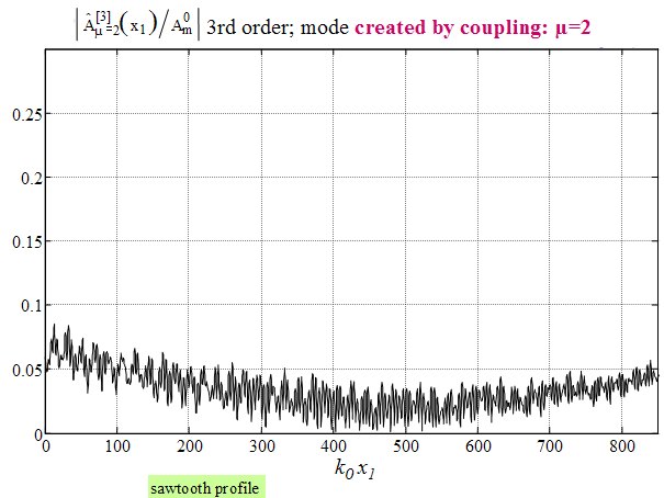 Figure 15 : Modulus of the acoustic pressure amplitude of the mode µ=2 created by coupling. The amplitude of this mode is much less important than those of modes µ=0 and
m=1, as it is predicted by the phonon relationship.
Click on the image for a zoom |
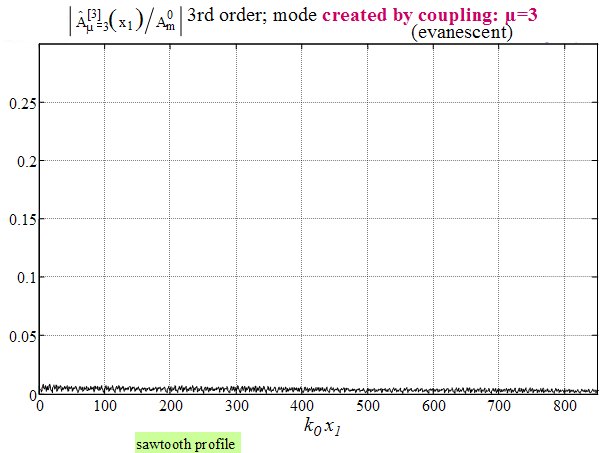 Figure 16 : Modulus of the acoustic pressure amplitude of the (evanescent) mode µ=3 created by coupling.
Click on the image for a zoom |
 Figure 17 : Modulus of the total acoustic pressure amplitude.
Click on the image for a zoom |
|
 Figure 18 : Dispersion
curves (red thick lines) of the smooth fluid waveguide and curves (blue
thin lines) corresponding to the phonon relationship.
Click on the image for a zoom |
Phonon relationship The
oscillation periods of the acoustic pressure amplitudes of
the different modes (figures 13-17), appear without any difficulty in the case of a
sinusoidal rough profile: phase terms and denominators of
the form
 This relation can be interpreted as a law of conservation of the phonon momentum in the dual space, leading to the term "phonon relationship".
The
red thick lines of figure 18 are the classical dispersion curves for guided
waves (with cut-off frequencies) for the four first modes. The blue thin lines
are the curves coming from the phonon relationship, for modes generated
by the source. The intersection between the two curves allow to predict when a strong self-coupling of the mode m=1 generated by the source with itself could occur (this is the case for example at fd/c0=1.26), or when a strong coupling of this mode m=1 with the mode µ=0 created by coupling (this occurs at fd/c0=1.31).
As these two frequencies are very closed to each other, it can easily be seen that, in the former example (figures 12-17),
there are both a strong self-coupling of the mode m=1 generated by the
source with itself, and a strong coupling of this mode m=1 with the mode
µ=0 created by coupling.
|
 Figure 19 : Intermodal couplings in the particular case of a symmetric sawtooth periodic profile. The modes created by coupling due to the roughness are denoted µ and the mode generated by the source is denoted m.
Click on the image for a zoom |
Intermodal couplings - Particular case of two symmetric (in phase) periodic sawtooth profiles (spatial period
) en dents de scieThe periodic profile (figure 19) consists of a regularly distribution of N small cavities (teeth) with a spatial period denoted
, on both sides of the guide (symmetric profile) .Four modes are taken into account here, the mode µ=3 being evanescent for the chosen frequency. The order n=3 is generally enough in order to make the model converge. The phonon relationships permit to predict either a strong or a weak coupling between the modes, and also the oscillation periods. |
 Figure 20 : Modulus of the acoustic pressure amplitude of the mode m=0 created by the source. The coupling due to the roughness creates other modes than the mode generated by the source, which leads to the decreasing of its acoustic pressure amplitude as a function of x1.
Click on the image for a zoom |
 Figure 21 : Modulus
of the acoustic pressure amplitude of the mode µ=1 created by
coupling. The amplitude of this mode is zero because m+µ=1
(odd).
Click on the image for a zoom |
 Figure 22 : Modulus
of the acoustic pressure amplitude of the mode µ=2 created by
coupling. The amplitude of this mode is much less important than that
of the mode m=0, as it can be predicted by the phonon relationship.
Click on the image for a zoom |
 Figure 23 : Modulus
of the acoustic pressure amplitude of the mode µ=3 created by coupling.
The amplitude of this mode is zero because m+µ=3 (odd).
Click on the image for a zoom |
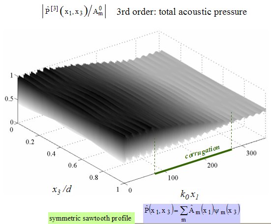 Figure 24 : Modulus of the total acoustic pressure amplitude.
Click on the image for a zoom |
 Under
construction...
Under
construction...
 Home page

